3  Model Development and Interpretation

This chapter is on the predictive models to look into the factors driving NYC traffic congestion.

3.1 Setup

Load the necessary libraries and preprocessed data:

Code
library(tidyverse)
library(tidymodels)
library(ranger) # For Random Forest
library(xgboost)
library(lightgbm)
library(lime)
library(iml) # For model-agnostic interpretations including SHAP
library(patchwork) # For combining plots
library(here)

# Set seed for reproducibility
set.seed(42)

3.2 Loading Preprocessed Data

Use the raw traffic CSV for modeling:

Code
# Load raw traffic data for modeling
model_data <- read_csv(here("data", "Automated_Traffic_Volume_Counts_20250505.csv"))
Rows: 1712605 Columns: 14
── Column specification ────────────────────────────────────────────────────────
Delimiter: ","
chr (6): Boro, WktGeom, street, fromSt, toSt, Direction
dbl (8): RequestID, Yr, M, D, HH, MM, Vol, SegmentID

ℹ Use `spec()` to retrieve the full column specification for this data.
ℹ Specify the column types or set `show_col_types = FALSE` to quiet this message.
Code
# Display structure
glimpse(model_data)
Rows: 1,712,605
Columns: 14
$ RequestID <dbl> 32970, 32970, 11342, 32970, 32970, 32970, 32970, 32970, 3297…
$ Boro      <chr> "Queens", "Queens", "Brooklyn", "Queens", "Queens", "Queens"…
$ Yr        <dbl> 2021, 2021, 2012, 2021, 2021, 2021, 2021, 2021, 2021, 2021, …
$ M         <dbl> 4, 4, 12, 4, 4, 4, 4, 4, 4, 4, 4, 4, 4, 4, 4, 4, 4, 4, 4, 4,…
$ D         <dbl> 30, 30, 18, 30, 30, 30, 30, 30, 30, 30, 30, 30, 30, 30, 30, …
$ HH        <dbl> 2, 2, 8, 2, 2, 3, 3, 3, 3, 4, 4, 4, 4, 5, 5, 5, 5, 6, 6, 6, …
$ MM        <dbl> 0, 15, 15, 30, 45, 0, 15, 30, 45, 0, 15, 30, 45, 0, 15, 30, …
$ Vol       <dbl> 0, 1, 33, 0, 0, 1, 0, 0, 1, 0, 0, 0, 1, 2, 4, 16, 5, 11, 9, …
$ SegmentID <dbl> 149701, 149701, 20063, 149701, 149701, 149701, 149701, 14970…
$ WktGeom   <chr> "POINT (997407.0998491726 208620.92612708386)", "POINT (9974…
$ street    <chr> "PULASKI BRIDGE", "PULASKI BRIDGE", "61 ST", "PULASKI BRIDGE…
$ fromSt    <chr> "Newtown Creek Shoreline", "Newtown Creek Shoreline", "15 AV…
$ toSt      <chr> "Dead end", "Dead end", "16 AV", "Dead end", "Dead end", "De…
$ Direction <chr> "NB", "NB", "WB", "NB", "NB", "NB", "NB", "NB", "NB", "NB", …

3.3 Data Preparation for Modeling

Split the data into training and testing sets, and prepare the feature set:

Code
# Function to prepare data for modeling
prepare_data_for_modeling <- function(df, target_col = "Vol", test_size = 0.2) {
  # Remove raw identifier columns not used in modeling
  features <- df %>%
    select(-c(Yr, M, D, HH, MM, Boro, WktGeom, street, fromSt, toSt))
  
  # Create the temporal split
  train_size <- floor((1 - test_size) * nrow(features))
  train_indices <- 1:train_size
  
  # Split data
  X_train <- features[train_indices, ] %>% select(-all_of(target_col))
  X_test <- features[-train_indices, ] %>% select(-all_of(target_col))
  y_train <- features[train_indices, ] %>% pull(target_col)
  y_test <- features[-train_indices, ] %>% pull(target_col)
  
  # Create recipe for preprocessing
  model_recipe <- recipe(~ ., data = X_train) %>%
    step_normalize(all_numeric_predictors())
  
  # Prepare the recipe
  model_prep <- prep(model_recipe)
  
  # Apply the recipe
  X_train_processed <- bake(model_prep, new_data = X_train)
  X_test_processed <- bake(model_prep, new_data = X_test)
  
  return(list(
    X_train = X_train,
    X_test = X_test,
    y_train = y_train,
    y_test = y_test,
    X_train_processed = X_train_processed,
    X_test_processed = X_test_processed,
    recipe = model_recipe
  ))
}

# Prepare data
model_data_split <- prepare_data_for_modeling(model_data)

# Check dimensions
cat("Training features:", dim(model_data_split$X_train), "\n")
Training features: 1370084 3 
Code
cat("Testing features:", dim(model_data_split$X_test), "\n")
Testing features: 342521 3 

3.4 Model Development

Train multiple models to predict traffic volume:

Code
# Function to train different models
train_models <- function(X_train, X_test, y_train, y_test, X_train_processed, X_test_processed) {
  models <- list()
  results <- list()
  
  # 1. Linear Regression (baseline)
  cat("Training Linear Regression...\n")
  lm_model <- linear_reg() %>%
    set_engine("lm") %>%
    fit(
      target ~ .,
      data = bind_cols(X_train_processed, target = y_train)
    )
  
  lm_preds <- predict(lm_model, new_data = X_test_processed)$.pred
  models[["Linear"]] <- lm_model
  
  # Calculate metrics
  lm_rmse <- sqrt(mean((lm_preds - y_test)^2))
  lm_r2 <- cor(lm_preds, y_test)^2
  
  results[["Linear"]] <- list(
    rmse = lm_rmse,
    r2 = lm_r2,
    feature_importance = lm_model$fit$coefficients[-1] # Exclude intercept
  )
  
  # 2. Random Forest
  cat("Training Random Forest...\n")
  rf_model <- rand_forest(trees = 100) %>%
    set_engine("ranger", importance = "impurity") %>%
    set_mode("regression") %>%
    fit(
      target ~ .,
      data = bind_cols(X_train, target = y_train)
    )
  
  rf_preds <- predict(rf_model, new_data = X_test)$.pred
  models[["RF"]] <- rf_model
  
  # Calculate metrics and feature importance
  rf_rmse <- sqrt(mean((rf_preds - y_test)^2))
  rf_r2 <- cor(rf_preds, y_test)^2
  rf_importance <- ranger::importance(rf_model$fit)
  
  results[["RF"]] <- list(
    rmse = rf_rmse,
    r2 = rf_r2,
    feature_importance = rf_importance
  )
  
  # 3. XGBoost
  cat("Training XGBoost...\n")
  # Convert character columns to numeric codes for XGBoost
  X_train_matrix <- X_train %>%
    mutate(across(where(is.character), ~ as.numeric(as.factor(.)))) %>%
    as.matrix()
  X_test_matrix <- X_test %>%
    mutate(across(where(is.character), ~ as.numeric(as.factor(.)))) %>%
    as.matrix()
  xgb_train <- xgb.DMatrix(data = X_train_matrix, label = y_train)
  xgb_test <- xgb.DMatrix(data = X_test_matrix, label = y_test)
  
  xgb_params <- list(
    objective = "reg:squarederror",
    eta = 0.1,
    max_depth = 6,
    nrounds = 100
  )
  
  xgb_model <- xgb.train(
    params = xgb_params,
    data = xgb_train,
    nrounds = 100,
    watchlist = list(train = xgb_train, test = xgb_test),
    verbose = 0
  )
  
  xgb_preds <- predict(xgb_model, xgb_test)
  models[["XGB"]] <- xgb_model
  
  # Calculate metrics and feature importance
  xgb_rmse <- sqrt(mean((xgb_preds - y_test)^2))
  xgb_r2 <- cor(xgb_preds, y_test)^2
  xgb_importance <- xgb.importance(model = xgb_model)
  
  results[["XGB"]] <- list(
    rmse = xgb_rmse,
    r2 = xgb_r2,
    feature_importance = setNames(xgb_importance$Gain, xgb_importance$Feature)
  )
  
  return(list(models = models, results = results))
}

# Train models
model_results <- train_models(
  model_data_split$X_train,
  model_data_split$X_test,
  model_data_split$y_train,
  model_data_split$y_test,
  model_data_split$X_train_processed,
  model_data_split$X_test_processed
)
Training Linear Regression...
Training Random Forest...
Training XGBoost...
[17:49:14] WARNING: src/learner.cc:767: 
Parameters: { "nrounds" } are not used.
Code
models <- model_results$models
results <- model_results$results

# Compare model performance
performance_df <- tibble(
  Model = names(results),
  RMSE = sapply(results, function(x) x$rmse),
  R2 = sapply(results, function(x) x$r2)
)

performance_df
# A tibble: 3 × 3
  Model   RMSE      R2
  <chr>  <dbl>   <dbl>
1 Linear  123. 0.00423
2 RF      106. 0.240  
3 XGB     102. 0.306  

3.5 Model Performance Visualization

Visualize the performance of the models:

Code
# Plot R² comparison
ggplot(performance_df, aes(x = Model, y = R2, fill = Model)) +
  geom_col() +
  scale_fill_brewer(palette = "Set2") +
  labs(
    title = "Model Performance Comparison (R² Score)",
    x = "Model",
    y = "R² Score"
  ) +
  ylim(0, 1) +
  theme_minimal() +
  theme(legend.position = "none")

# Plot RMSE comparison
ggplot(performance_df, aes(x = Model, y = RMSE, fill = Model)) +
  geom_col() +
  scale_fill_brewer(palette = "Set2") +
  labs(
    title = "Model Performance Comparison (RMSE)",
    x = "Model",
    y = "RMSE"
  ) +
  theme_minimal() +
  theme(legend.position = "none")

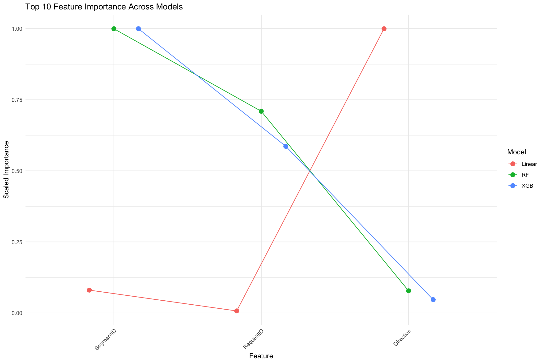
3.6 Feature Importance Analysis

Feature importance across the different models:

Code
# Determine original feature list from Random Forest results
original_feats <- names(results$RF$feature_importance)
feature_importance_df <- tibble(Feature = original_feats)

# Linear model: aggregate dummy coefficients by original feature
linear_coefs <- results$Linear$feature_importance
feature_importance_df$Linear <- sapply(original_feats, function(f) {
  matched <- grep(paste0('^', f), names(linear_coefs), value = TRUE)
  if (length(matched) == 0) {
    0
  } else {
    sum(abs(linear_coefs[matched]))
  }
})

# Other models: ensure each feature has an importance (zero if missing)
for (model_name in setdiff(names(results), 'Linear')) {
  imp_vec <- results[[model_name]]$feature_importance
  feature_importance_df[[model_name]] <- sapply(original_feats, function(f) {
    if (f %in% names(imp_vec)) imp_vec[[f]] else 0
  })
}

# Scale importance scores to 0-1 range for comparison
for (model_name in names(results)) {
  max_val <- max(feature_importance_df[[model_name]])
  feature_importance_df[[model_name]] <- feature_importance_df[[model_name]] / max_val
}

# Calculate mean importance
feature_importance_df <- feature_importance_df %>%
  mutate(
    Mean_Importance = rowMeans(select(., -Feature)),
    # Add feature ranks
    Mean_Rank = rank(-Mean_Importance)
  ) %>%
  arrange(Mean_Rank)

# Top features
top_n_features <- 10
top_features <- feature_importance_df %>%
  top_n(top_n_features, Mean_Importance) %>%
  pull(Feature)

# Reshape for plotting
importance_long <- feature_importance_df %>%
  filter(Feature %in% top_features) %>%
  pivot_longer(
    cols = c(-Feature, -Mean_Importance, -Mean_Rank),
    names_to = "Model",
    values_to = "Importance"
  )

# Plot top features
ggplot(importance_long, aes(x = reorder(Feature, -Mean_Importance), y = Importance, color = Model)) +
  geom_point(size = 3, position = position_dodge(width = 0.5)) +
  geom_line(aes(group = Model), position = position_dodge(width = 0.5)) +
  labs(
    title = paste("Top", top_n_features, "Feature Importance Across Models"),
    x = "Feature",
    y = "Scaled Importance"
  ) +
  theme_minimal() +
  theme(axis.text.x = element_text(angle = 45, hjust = 1))

3.7 SHAP Value Analysis

Code
# Create an explainer using the iml package
X_test_matrix <- as.matrix(model_data_split$X_test)
predictor <- Predictor$new(
  model = models$XGB, 
  data = X_test_matrix, 
  y = model_data_split$y_test,
  type = "regression"
)

# Compute SHAP values
system.time({
  shapley <- Shapley$new(predictor, x.interest = X_test_matrix[1, ])
})

# Plot SHAP values for a single instance
plot(shapley)

# For a more comprehensive view, we can calculate SHAP values for multiple instances
# This is computationally intensive, so we'll sample a small number
sample_indices <- sample(1:nrow(X_test_matrix), 100)
sampled_X_test <- X_test_matrix[sample_indices, ]

# Feature effects using partial dependence
feature_effects <- FeatureEffects$new(predictor, features = top_features)
plot(feature_effects)

# Feature importance based on SHAP
feature_importance <- FeatureImp$new(predictor, loss = "mse")
plot(feature_importance)

3.8 LIME Analysis

Code
# Create a LIME explainer
lime_explainer <- lime(
  x = as.data.frame(model_data_split$X_train),
  model = function(x) {
    pred <- predict(models$XGB, as.matrix(x))
    data.frame(Prediction = pred)
  },
  bin_continuous = TRUE,
  quantile_bins = FALSE,
  n_bins = 5
)

# Select a few samples to explain
sample_to_explain <- model_data_split$X_test[sample(nrow(model_data_split$X_test), 5), ]

# Generate explanations
lime_explanations <- lime::explain(
  x = sample_to_explain,
  explainer = lime_explainer,
  n_features = 10,
  feature_select = "highest_weights"
)

# Plot LIME explanations
plot_lime <- plot_explanations(lime_explanations) +
  labs(title = "LIME Explanations for Sample Predictions")

plot_lime

3.9 Stability Analysis

Code
# Function for stability analysis
perform_stability_analysis <- function(df, n_iterations = 10) {
  
  cat("Performing stability analysis...\n")
  # Initialize dataframes to store feature importance ranks
  all_features <- colnames(df %>% select(-c(Vol, Date, Year, Month, Day, Boro)))
  
  rf_ranks <- matrix(NA, nrow = length(all_features), ncol = n_iterations)
  rownames(rf_ranks) <- all_features
  
  xgb_ranks <- matrix(NA, nrow = length(all_features), ncol = n_iterations)
  rownames(xgb_ranks) <- all_features
  
  # Multiple iterations with different data splits
  for (i in 1:n_iterations) {
    cat(sprintf("Stability iteration %d/%d\n", i, n_iterations))
    
    # Sample 80% of the data
    sample_indices <- sample(1:nrow(df), size = floor(0.8 * nrow(df)))
    sample_df <- df[sample_indices, ]
    
    # Prepare data
    X <- sample_df %>% select(-c(Vol, Date, Year, Month, Day, Boro))
    y <- sample_df$Vol
    
    # Split data
    train_indices <- sample(1:nrow(X), size = floor(0.8 * nrow(X)))
    X_train <- X[train_indices, ]
    X_test <- X[-train_indices, ]
    y_train <- y[train_indices]
    y_test <- y[-train_indices]
    
    # Train Random Forest
    rf_model <- ranger(
      y ~ .,
      data = bind_cols(X_train, y = y_train),
      importance = "impurity",
      num.trees = 100
    )
    
    # Train XGBoost
    xgb_train <- xgb.DMatrix(as.matrix(X_train), label = y_train)
    xgb_model <- xgb.train(
      params = list(objective = "reg:squarederror", eta = 0.1, max_depth = 6),
      data = xgb_train,
      nrounds = 100,
      verbose = 0
    )
    
    # Extract feature importance
    rf_importance <- ranger::importance(rf_model)
    rf_ranked <- rank(-rf_importance)
    
    xgb_importance <- xgb.importance(model = xgb_model)
    xgb_ranked <- rep(NA, length(all_features))
    names(xgb_ranked) <- all_features
    xgb_ranked[xgb_importance$Feature] <- rank(-xgb_importance$Gain)
    
    # Store ranks
    rf_ranks[, i] <- rf_ranked
    xgb_ranks[, i] <- xgb_ranked
  }
  
  # Calculate stability metrics
  rf_mean_rank <- rowMeans(rf_ranks, na.rm = TRUE)
  rf_std_rank <- apply(rf_ranks, 1, sd, na.rm = TRUE)
  xgb_mean_rank <- rowMeans(xgb_ranks, na.rm = TRUE)
  xgb_std_rank <- apply(xgb_ranks, 1, sd, na.rm = TRUE)
  
  # Combine results
  stability_results <- tibble(
    Feature = all_features,
    RF_Mean_Rank = rf_mean_rank,
    RF_Std_Rank = rf_std_rank,
    XGB_Mean_Rank = xgb_mean_rank,
    XGB_Std_Rank = xgb_std_rank
  ) %>%
    mutate(
      Avg_Rank = (RF_Mean_Rank + XGB_Mean_Rank) / 2
    ) %>%
    arrange(Avg_Rank)
  
  return(stability_results)
}

# Run stability analysis
stability_results <- perform_stability_analysis(model_data)

# Plot stability results
top_features_stability <- stability_results %>%
  top_n(10, -Avg_Rank) %>%
  pull(Feature)

stability_plot <- stability_results %>%
  filter(Feature %in% top_features_stability) %>%
  ggplot(aes(x = reorder(Feature, -Avg_Rank))) +
  geom_point(aes(y = RF_Mean_Rank, color = "Random Forest"), size = 3) +
  geom_errorbar(
    aes(ymin = RF_Mean_Rank - RF_Std_Rank, ymax = RF_Mean_Rank + RF_Std_Rank, color = "Random Forest"),
    width = 0.2
  ) +
  geom_point(aes(y = XGB_Mean_Rank, color = "XGBoost"), size = 3) +
  geom_errorbar(
    aes(ymin = XGB_Mean_Rank - XGB_Std_Rank, ymax = XGB_Mean_Rank + XGB_Std_Rank, color = "XGBoost"),
    width = 0.2
  ) +
  labs(
    title = "Feature Importance Stability Analysis",
    x = "Feature",
    y = "Mean Rank (lower is more important)",
    color = "Model"
  ) +
  theme_minimal() +
  theme(axis.text.x = element_text(angle = 45, hjust = 1))

stability_plot

3.10 Interpretability Method Comparison

Code
# Combine all importance rankings
all_methods_comparison <- tibble(
  Feature = feature_importance_df$Feature,
  Standard_Importance = feature_importance_df$Mean_Rank,
  SHAP_Rank = NA, # We'll populate this from feature_importance object if available
  LIME_Rank = NA # This would come from aggregate LIME results
)

# If SHAP analysis was run, extract feature rankings
if (exists("feature_importance")) {
  shap_importance_df <- as.data.frame(feature_importance$results)
  
  # Match features between datasets
  for (i in 1:nrow(all_methods_comparison)) {
    feature <- all_methods_comparison$Feature[i]
    matching_row <- which(shap_importance_df$feature == feature)
    
    if (length(matching_row) > 0) {
      all_methods_comparison$SHAP_Rank[i] <- shap_importance_df$importance[matching_row]
    }
  }
  
  # Convert to ranks
  all_methods_comparison$SHAP_Rank <- rank(-all_methods_comparison$SHAP_Rank)
}

# Calculate Spearman correlation between methods
corr_matrix <- cor(
  all_methods_comparison %>% 
    select(-Feature) %>% 
    select_if(~!all(is.na(.))), 
  method = "spearman",
  use = "pairwise.complete.obs"
)

# Display correlation matrix
print(corr_matrix)

# Visualize method agreement for top features
top_method_features <- all_methods_comparison %>%
  filter(Feature %in% top_features) %>%
  pivot_longer(
    cols = c(-Feature),
    names_to = "Method",
    values_to = "Rank"
  ) %>%
  filter(!is.na(Rank))

# Plot comparison
ggplot(top_method_features, aes(x = reorder(Feature, -Rank), y = Rank, color = Method)) +
  geom_point(size = 3, position = position_dodge(width = 0.5)) +
  geom_line(aes(group = Method), position = position_dodge(width = 0.5)) +
  labs(
    title = "Comparison of Feature Rankings Across Interpretability Methods",
    x = "Feature",
    y = "Rank (lower is more important)"
  ) +
  theme_minimal() +
  theme(axis.text.x = element_text(angle = 45, hjust = 1))

3.11 Summary

  1. Developed multiple predictive models for NYC traffic volume, including Linear Regression, Random Forest, and XGBoost
  2. Applied interpretability methods including feature importance, SHAP, and LIME to understand model decisions
  3. Conducted stability analysis to assess the robustness of feature importance rankings
  4. Compared interpretability methods to identify consistent patterns in feature importance

The next chapter will present detailed results and insights from these analyses, focusing on the key factors influencing NYC traffic congestion.