2.1 Data Processing

::: {.cell}

Code
library(tidyverse)
library(lubridate)
library(ggplot2)
library(scales)
library(here)

:::

2.1.1 Weather Data Preprocessing

Code
# Set file paths
weather_temp_path <- here("data", "monthly_nyc_weather.csv")
weather_rain_path <- here("data", "monthly_nyc_rain.csv")

# Function to preprocess weather data
preprocess_weather_data <- function() {
  # Load temperature and rainfall data
  temp_df <- read_csv(weather_temp_path)
  rain_df <- read_csv(weather_rain_path)
  
  # Convert Month format to date
  temp_df <- temp_df %>%
    mutate(Date = as.Date(paste0(Month, "01"), format = "%Y%m%d"))
  
  rain_df <- rain_df %>%
    mutate(Date = as.Date(paste0(Month, "01"), format = "%Y%m%d"))
  
  # Rename columns for clarity
  temp_df <- temp_df %>%
    rename(Temperature = Value, TempAnomaly = Anomaly)
  
  rain_df <- rain_df %>%
    rename(Rainfall = Value, RainAnomaly = Anomaly)
  
  # Merge temperature and rainfall data
  weather_df <- temp_df %>%
    inner_join(rain_df, by = c("Date"))
  
  # Extract date components for analysis
  weather_df <- weather_df %>%
    mutate(
      Year = year(Date),
      Month = month(Date),
      # Create season feature
      Season = case_when(
        Month %in% c(12, 1, 2) ~ "Winter",
        Month %in% c(3, 4, 5) ~ "Spring",
        Month %in% c(6, 7, 8) ~ "Summer",
        TRUE ~ "Fall"
      )
    )
  
  return(weather_df)
}

# Process weather data
weather_df <- preprocess_weather_data()
Rows: 147 Columns: 3
── Column specification ────────────────────────────────────────────────────────
Delimiter: ","
dbl (3): Month, Value, Anomaly

ℹ Use `spec()` to retrieve the full column specification for this data.
ℹ Specify the column types or set `show_col_types = FALSE` to quiet this message.
Rows: 147 Columns: 3
── Column specification ────────────────────────────────────────────────────────
Delimiter: ","
dbl (3): Month, Value, Anomaly

ℹ Use `spec()` to retrieve the full column specification for this data.
ℹ Specify the column types or set `show_col_types = FALSE` to quiet this message.
Code
# Display the first few rows
head(weather_df)
# A tibble: 6 × 10
  Month.x Temperature TempAnomaly Date       Month.y Rainfall RainAnomaly  Year
    <dbl>       <dbl>       <dbl> <date>       <dbl>    <dbl>       <dbl> <dbl>
1  201301        35.1         1.3 2013-01-01  201301     2.76       -0.7   2013
2  201302        33.9        -2.1 2013-02-01  201302     4.25        0.48  2013
3  201303        40.1        -1.7 2013-03-01  201303     2.89       -0.93  2013
4  201304        53          -0.2 2013-04-01  201304     1.31       -2.63  2013
5  201305        62.8        -0.8 2013-05-01  201305     8           3.45  2013
6  201306        72.7         0.5 2013-06-01  201306    10.1         5.5   2013
# ℹ 2 more variables: Month <dbl>, Season <chr>

2.1.2 Traffic Data Preprocessing

Code
traffic_path <- here("data", "Automated_Traffic_Volume_Counts_20250505.csv")

# Function to preprocess traffic data
preprocess_traffic_data <- function(sample_size = NULL) {
  # Load traffic data with sampling if needed due to size
  if (!is.null(sample_size)) {
    traffic_df <- read_csv(traffic_path, n_max = sample_size)
  } else {
    traffic_df <- read_csv(traffic_path)
  }
  
  # Handle missing values
  traffic_df <- traffic_df %>%
    filter(!is.na(Vol))
  
  # Create datetime column and extract components
  traffic_df <- traffic_df %>%
    mutate(
      DateTime = as.POSIXct(paste(Yr, M, D, HH, MM, sep = "-"), format = "%Y-%m-%d-%H-%M"),
      Year = year(DateTime),
      Month = month(DateTime),
      Day = day(DateTime),
      DayOfWeek = wday(DateTime) - 1,  # 0 = Sunday, 6 = Saturday
      Hour = hour(DateTime),
      
      # Create features for time of day
      TimeOfDay = case_when(
        Hour >= 6 & Hour < 10 ~ "Morning",
        Hour >= 10 & Hour < 16 ~ "Midday",
        Hour >= 16 & Hour < 20 ~ "Evening",
        TRUE ~ "Night"
      ),
      
      # Create weekday/weekend feature
      IsWeekend = if_else(DayOfWeek >= 5, 1, 0)
    )
  
  return(traffic_df)
}

# Process traffic data (with sampling due to large file size)
traffic_df <- preprocess_traffic_data(sample_size = 100000)

# Show summary
summary(traffic_df)

2.1.3 Emergency Response Data Preprocessing

Code
emergency_path <- here("data", "911_Open_Data_Local_Law_119_20250505.csv")

# Function to preprocess emergency response data
preprocess_emergency_data <- function() {
  emergency_df <- read_csv(emergency_path)
  
  # Extract date from 'Month Name' column
  emergency_df <- emergency_df %>%
    mutate(
      Date = as.Date(paste0("01 ", `Month Name`), format = "%d %Y / %m"),
      Year = year(Date),
      Month = month(Date)
    )
  
  return(emergency_df)
}

# Process emergency data
emergency_df <- preprocess_emergency_data()
Rows: 10166 Columns: 6
── Column specification ────────────────────────────────────────────────────────
Delimiter: ","
chr (4): Month Name, Agency, Description, Borough
dbl (2): # of Incidents, Response Times

ℹ Use `spec()` to retrieve the full column specification for this data.
ℹ Specify the column types or set `show_col_types = FALSE` to quiet this message.
Code
# Display the structure
glimpse(emergency_df)
Rows: 10,166
Columns: 9
$ `Month Name`     <chr> "2025 / 03", "2025 / 03", "2025 / 03", "2025 / 03", "…
$ Agency           <chr> "Aggregate", "Aggregate", "Aggregate", "Aggregate", "…
$ Description      <chr> "Combined average response time to life threatening m…
$ Borough          <chr> "Brooklyn", "Bronx", "Manhattan", "Queens", "Staten I…
$ `# of Incidents` <dbl> 13615, 11039, 10868, 9819, 2398, 59, 601, 12750, 2732…
$ `Response Times` <dbl> 567.01, 683.05, 642.23, 601.25, 550.99, 849.32, 515.4…
$ Date             <date> 2025-03-01, 2025-03-01, 2025-03-01, 2025-03-01, 2025…
$ Year             <dbl> 2025, 2025, 2025, 2025, 2025, 2025, 2025, 2025, 2025,…
$ Month            <dbl> 3, 3, 3, 3, 3, 3, 3, 3, 3, 3, 3, 3, 3, 3, 3, 3, 3, 3,…

2.2 Exploratory Data Analysis

Code
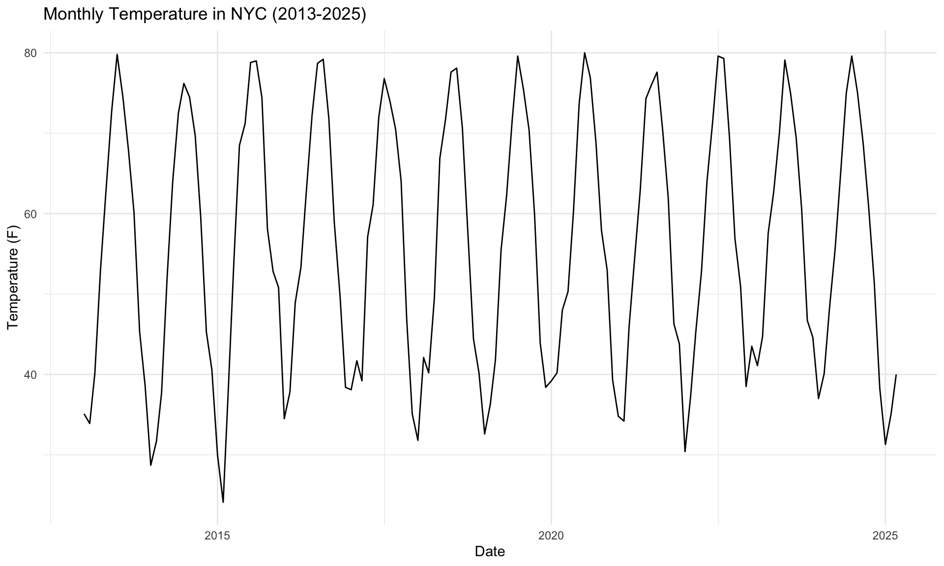
# 1. Weather patterns over time
ggplot(weather_df, aes(x = Date, y = Temperature)) +
  geom_line() +
  labs(
    title = "Monthly Temperature in NYC (2013-2025)",
    x = "Date",
    y = "Temperature (F)"
  ) +
  theme_minimal()

Code
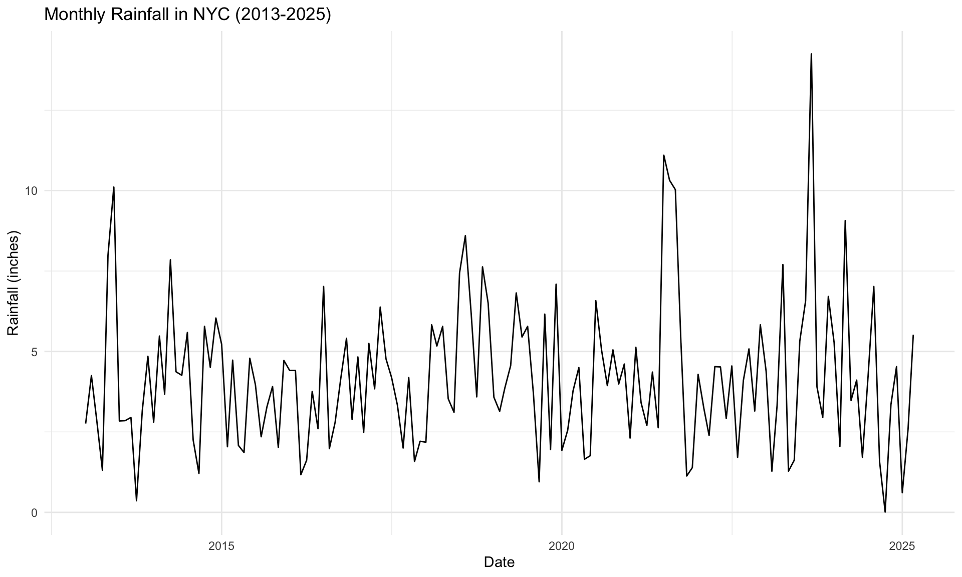
ggplot(weather_df, aes(x = Date, y = Rainfall)) +
  geom_line() +
  labs(
    title = "Monthly Rainfall in NYC (2013-2025)",
    x = "Date",
    y = "Rainfall (inches)"
  ) +
  theme_minimal()

Code
# Traffic volume by time of day
traffic_df %>%
  group_by(TimeOfDay) %>%
  summarize(MeanVolume = mean(Vol, na.rm = TRUE)) %>%
  mutate(TimeOfDay = factor(TimeOfDay, levels = c("Morning", "Midday", "Evening", "Night"))) %>%
  ggplot(aes(x = TimeOfDay, y = MeanVolume)) +
  geom_col(fill = "steelblue") +
  labs(
    title = "Average Traffic Volume by Time of Day",
    x = "Time of Day",
    y = "Average Volume"
  ) +
  theme_minimal()

# Traffic volume by borough
traffic_df %>%
  group_by(Boro) %>%
  summarize(MeanVolume = mean(Vol, na.rm = TRUE)) %>%
  arrange(desc(MeanVolume)) %>%
  ggplot(aes(x = reorder(Boro, MeanVolume), y = MeanVolume)) +
  geom_col(fill = "steelblue") +
  labs(
    title = "Average Traffic Volume by Borough",
    x = "Borough",
    y = "Average Volume"
  ) +
  theme_minimal() +
  coord_flip()
Code
# Emergency response times by borough
ggplot(emergency_df, aes(x = Borough, y = `Response Times`)) +
  geom_boxplot(fill = "steelblue", alpha = 0.7) +
  labs(
    title = "Emergency Response Times by Borough",
    x = "Borough",
    y = "Response Time (seconds)"
  ) +
  theme_minimal() +
  theme(axis.text.x = element_text(angle = 45, hjust = 1))

2.3 Data Integration

Code
# Function to integrate datasets
integrate_datasets <- function(traffic_df, weather_df, emergency_df) {
  # Aggregate traffic data to daily level
  daily_traffic <- traffic_df %>%
    group_by(Year, Month, Day, Boro) %>%
    summarize(Vol = mean(Vol, na.rm = TRUE), .groups = "drop") %>%
    mutate(Date = as.Date(paste(Year, Month, Day, sep = "-")))
  
  # Expand weather data to daily
  weather_expanded <- weather_df %>%
    select(Date, Temperature, Rainfall, TempAnomaly, RainAnomaly, Season) %>%
    mutate(
      month_start = floor_date(Date, "month"),
      month_end = ceiling_date(Date, "month") - days(1)
    )
  
  # Create daily weather records
  daily_weather_records <- list()
  
  for (i in 1:nrow(weather_expanded)) {
    row <- weather_expanded[i, ]
    date_range <- seq(row$month_start, row$month_end, by = "day")
    
    for (date in date_range) {
      daily_record <- row
      daily_record$Date <- date
      daily_weather_records[[length(daily_weather_records) + 1]] <- daily_record
    }
  }
  
  daily_weather <- bind_rows(daily_weather_records) %>%
    select(-month_start, -month_end)
  
  # Merge daily traffic with daily weather
  merged_df <- daily_traffic %>%
    inner_join(daily_weather, by = "Date") %>%
    mutate(
      DayOfWeek = wday(Date) - 1,
      IsWeekend = if_else(DayOfWeek >= 5, 1, 0)
    )
  
  return(merged_df)
}

# Integrate datasets
integrated_data <- integrate_datasets(traffic_df, weather_df, emergency_df)

# Save processed data
write_csv(weather_df, here("data", "processed_weather_data.csv"))
write_csv(traffic_df, here("data", "processed_traffic_data.csv"))
write_csv(emergency_df, here("data", "processed_emergency_data.csv"))
write_csv(integrated_data, here("data", "integrated_data.csv"))

# Display the structure of the integrated dataset
glimpse(integrated_data)

2.4 Feature Engineering

Code
# Function to engineer features
engineer_features <- function(df) {
  # One-hot encode categorical variables
  df <- df %>%
    mutate(
      Season_Spring = if_else(Season == "Spring", 1, 0),
      Season_Summer = if_else(Season == "Summer", 1, 0),
      Season_Fall = if_else(Season == "Fall", 1, 0),
      Season_Winter = if_else(Season == "Winter", 1, 0)
    )
  
  # Create borough dummy variables
  boroughs <- unique(df$Boro)
  for (borough in boroughs) {
    col_name <- paste0("Boro_", borough)
    df[[col_name]] <- if_else(df$Boro == borough, 1, 0)
  }
  
  # Add lagged features (previous day's traffic volume)
  for (borough in boroughs) {
    col_name <- paste0("Boro_", borough)
    lag_col_name <- paste0(borough, "_prev_day_vol")
    
    # Filter for this borough and sort by date
    boro_data <- df %>%
      filter(!!sym(col_name) == 1) %>%
      arrange(Date)
    
    # Create lagged volume
    boro_data <- boro_data %>%
      mutate(!!lag_col_name := lag(Vol))
    
    # Update the original dataframe
    df <- df %>%
      left_join(
        boro_data %>% select(Date, Boro, !!lag_col_name),
        by = c("Date", "Boro")
      )
  }
  
  # Fill NA values from lagged features with mean values
  for (col in names(df)) {
    if (any(is.na(df[[col]]))) {
      col_mean <- mean(df[[col]], na.rm = TRUE)
      df[[col]] <- if_else(is.na(df[[col]]), col_mean, df[[col]])
    }
  }
  
  return(df)
}

# Engineer features
engineered_data <- engineer_features(integrated_data)

# Save engineered data
write_csv(engineered_data, here("data", "engineered_data.csv"))

# Summary of engineered features
summary(engineered_data)

2.5 Summary

  1. Loaded and cleaned three distinct datasets: traffic volumes, weather patterns, and emergency response times
  2. Created time-based features including time of day, day of week, and seasonal indicators
  3. Performed exploratory visualizations to understand traffic patterns by time and location
  4. Integrated the datasets to create a comprehensive view of NYC traffic patterns
  5. Engineered additional features to improve the model’s predictive capabilities

The prepared data will be called in the next chapter to develop the models and analysis.